查询处理¶

约 3765 个字 10 行代码 23 张图片预计阅读时间 19 分钟

Basic Steps in Query Processing¶

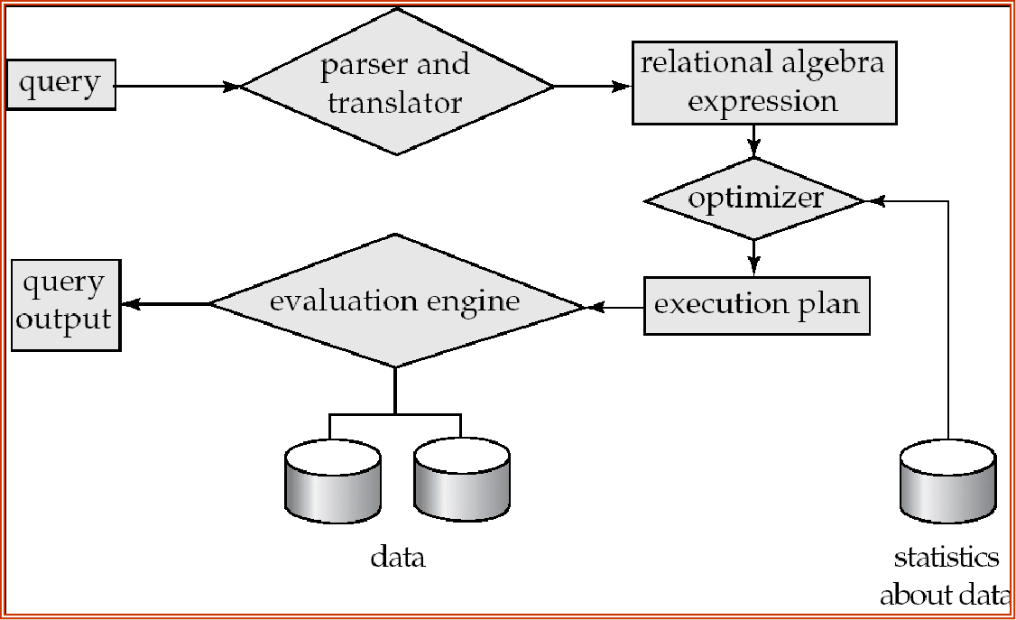
查询处理的基本步骤是：

解析与转换 (Parsing and translation)
- 将查询转换为其内部形式，通常转换为关系代数形式
- 解析器执行以下任务：
  - 检查查询的语法是否正确
  - 验证查询中引用的关系是否存在
  - 检查属性名是否有效
优化 (Optimization)
- 在所有等价的执行计划中，选择代价最低的执行计划
- 查询优化器负责生成有效的查询执行计划
执行 (Evaluation)
- 查询执行引擎接收查询执行计划
- 按照计划执行各个操作
- 返回查询结果给用户

🌰

对于如下的语句:

select name, title 
from instructor natural join (teaches natural join course)
where dept_name=‘Music’ and year = 2009;

用关系代数来表达就是: $$ \pi_{name,title}(\sigma_{dept_name=‘Music’ \land year=2009}(instructor \bowtie (teaches \bowtie course))) $$

优化前与优化后的表达树为:

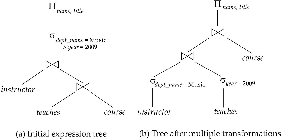
从中可以看出几点逻辑:

把选择运算往叶子上推；因为叶子节点的表小，选择运算的代价小，并且这样也能减少中间结果集的大小。
小的表先连接，减少中间结果集的大小。

An evaluation plan defines exactly what algorithm is used for each operation, and how the execution of the operations is coordinated.

如下图:

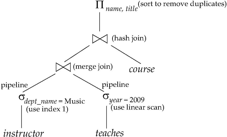
左边使用B+树扫描，右边使用线性扫描，并且两边是可以Pipeline的。

还有merge join和hash join的区别。

Measurement of Query Cost¶

Typically disk access is the predominant cost, and is also relatively easy to estimate.

硬盘访问的开销总是最大的

我们考虑如下三个因素:

Number of seeks
Number of blocks read
Number of blocks written

通常写的代价比读大很多，因为一般写完我们还要读一遍来检验。

为了简化，我们使用如下两个量来评估代价:

number of block transfers,与之相配的是$t_T$ – time to transfer one block
number of seeks,与之相配的是$t_S$ – time to perform one seek
对于b次块传输和s次寻道，代价为： $$ C = b \cdot t_T + s \cdot t_S$$

We often use worst case estimates, assuming only the minimum amount of memory needed for the operation is available

Selection Operation¶

File scan¶

Algorithm A1 (linear search). Scan each file block and test all records to see whether they satisfy the selection condition.

我们假定块是连续存放的

Worst Cost:$b_r \times t_T + t_S$
- $b_r$是块数目
Average Cost: $\frac{b_r}{2} \times t_T + t_S$
- 如果查找的是一个主键值，并且我们找到符合的就停止

Index scan¶

search algorithms that use an index

A2¶

A2 (primary B+-tree index / clustering B+-tree index, equality on key).

即使用B+树索引
找的是主键值

Cost:

\[ C = (t_S + t_T) \cdot (h + 1)\]

$h$是树的高度
B+树每到新的一层,都要重新寻道一次
最后要+1是因为我们要读数据块

A3¶

A3 (primary B+-tree index/ clustering B+-tree index, equality on nonkey)

即使用B+树索引
找的是非主键值
所以可能有多个结果

Records will be on consecutive blocks, 所以最后找数据块只需要寻道一次

Let b = number of blocks containing matching records

Cost:

\[ C = (t_S + t_T) \cdot h + t_S+ b \cdot t_T\]

A4¶

A4 (secondary B+-tree index , equality on key)

即使用B+树索引
找的是主键值
但使用的是非聚集索引

Cost和A2一样:

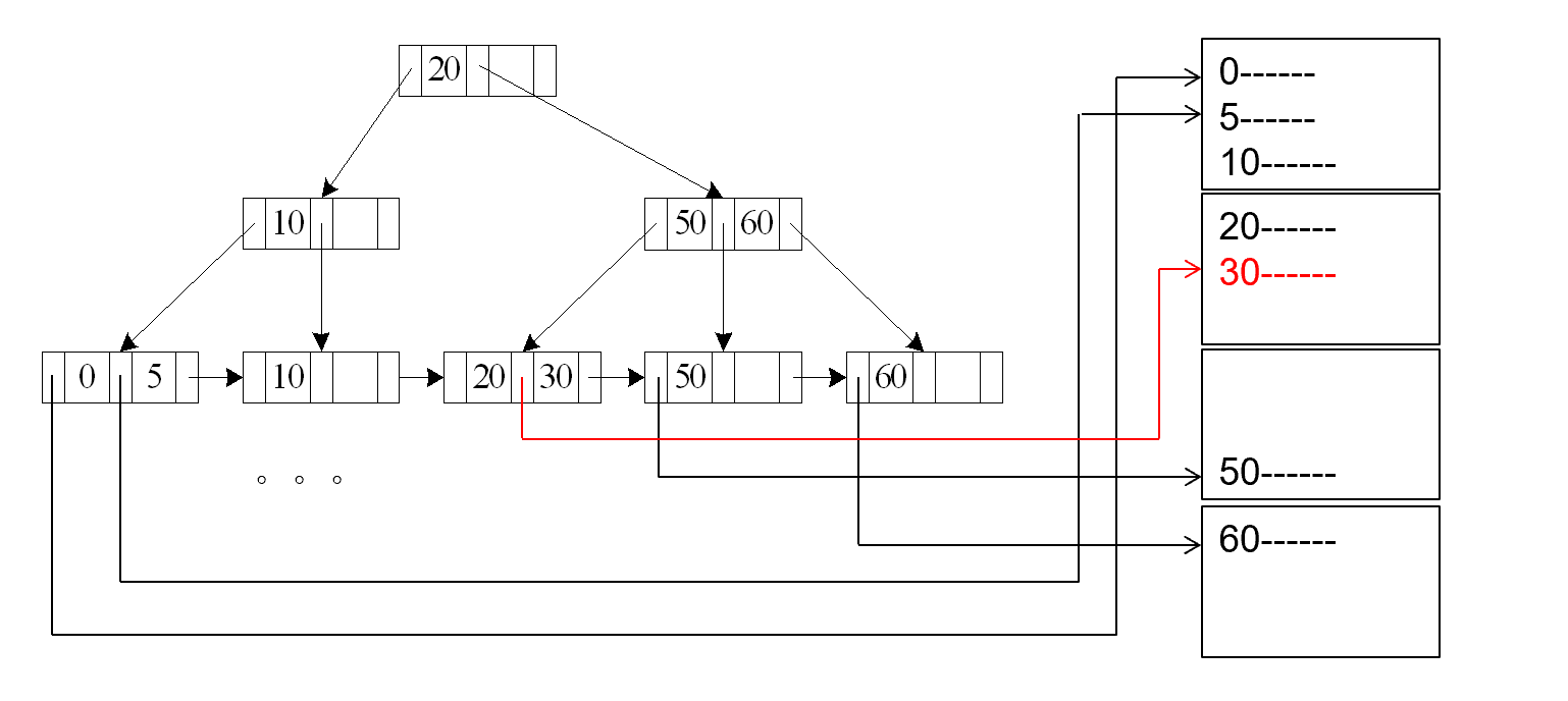
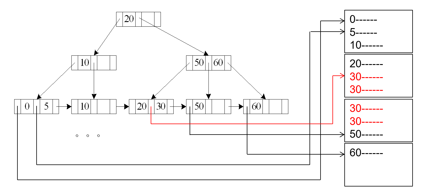
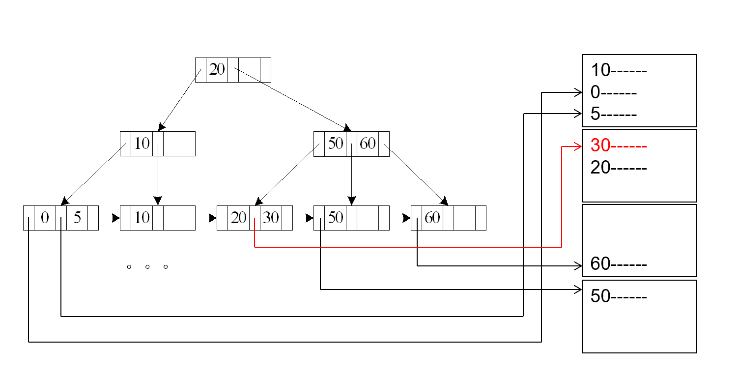
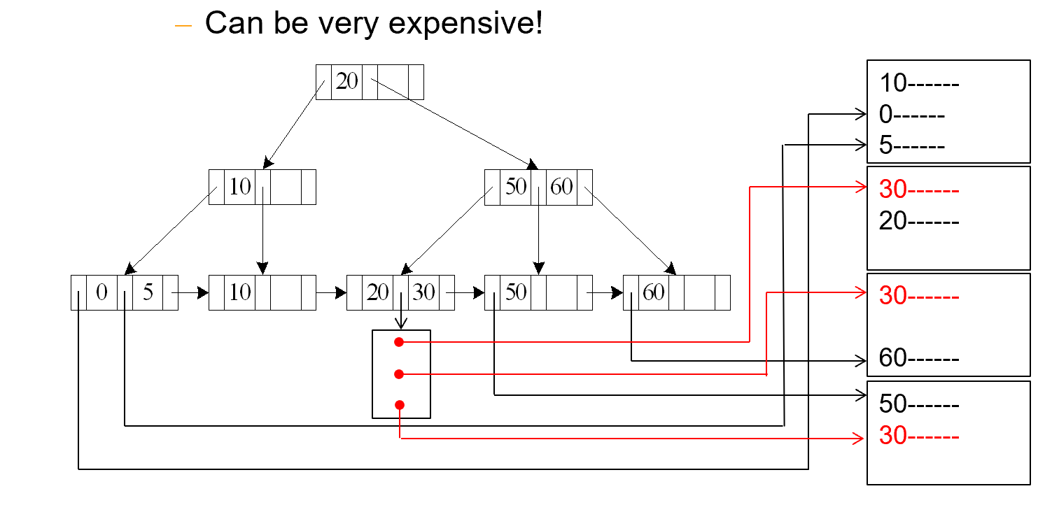
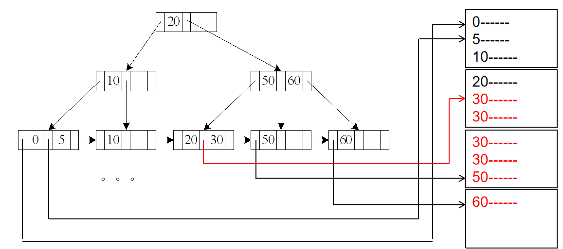
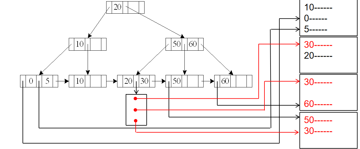
A4'¶

A4' (secondary B+-tree index , equality on nonkey)

即使用B+树索引
找的是非主键值
使用的是非聚集索引

m 表示放指针的块的数量

n 表示对应磁盘里的记录的数量。

\[ Cost = (t_S + t_T) \cdot (h + m + n) \]

Selections Involving Comparisons¶

进行查找$\sigma_{A \leq B}(r)$或$\sigma_{A \geq B}(r)$

A5¶

A5 (primary B+-index / clustering B+-index index, comparison)

索引是主键值
包含比较
已经排好序
对于$\sigma_{A \geq B}(r)$
- 先找到第一个符合的值，然后顺序扫描
- Cost和A3一样
对于$\sigma_{A \leq B}(r)$
- 不需要使用索引
- 直接从数据块里顺序扫描，直到读到第一个元组大于B为止

A6¶

A6 (secondary B+-tree index, comparison)

对于$\sigma_{A \geq B}(r)$
- 根据B+树索引找到第一个符合的值，然后顺序扫描
对于$\sigma_{A \leq B}(r)$
- 直接在叶子节点逐个扫描，直到读到第一个元组大于B为止
- 然后对于每一个指针，去数据块里顺序读

Implementation of Complex Selections¶

对于多条件的选择:$\sigma_{\theta_1 \land \theta_2 \land ... \land \theta_n}(r)$

A7 (conjunctive selection using one index)
- 选一个条件，从A1-A6之间找一个最优的算法，得到一堆元组
- 在这堆元组上测试其他条件
A8 (conjunctive selection using composite index)
- Use appropriate composite (multiple-key) index if available.
A9 (conjunctive selection by intersection of identifiers)
- 对于每一个条件，从A1-A6中选择一个最优的算法，得到结果集
- 把结果集取交

Algorithms for Complex Selections¶

对于多条件的选择:$\sigma_{\theta_1 \lor \theta_2 \lor ... \lor \theta_n}(r)$
- Applicable if all conditions have available indices.
- Otherwise use linear scan.
- Use corresponding index for each condition, and take union of all the obtained sets of record pointers.
- Then fetch records from file
取反的选择:$\sigma_{\neg \theta}(r)$
- 先用线性扫描找出所有的元组，然后在内存中进行选择

Bitmap¶

没讲

Sorting¶

和ADS中的外部排序很像,但是我当时没写(悲)

Runs 与 Pass

为了避免模糊，在这里直接把这两个关键定义给出

Run:一组已经排序好的数据，初始的Runs大小和内存大小一致
Pass:一个把N个Runs归并排序为$\frac{N}{M}$个Runs,其中M是内存中可以放的Block数量。

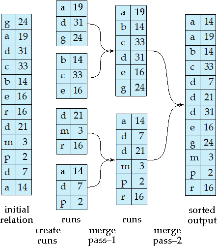
排序步骤¶

Create sorted runs(归并段 )
- Let i be 0 initially.
- Repeatedly do the following till the end of the relation:
  - Read M blocks of relation into memory
  - Sort the in-memory blocks
  - Write sorted data to run $R_i$; increment
  - Let the final value of i be N
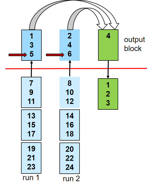
Merge the runs (N-way merge)
- $N \leq M$
  - 那么只需要一个Pass
  - 为每一个run准备一个Block作为缓冲区，再来一个Block作为输出的缓冲区，从每个run中读一个Block到缓冲区
  - 重复以下过程直到结束:
    - 对于缓冲区里面所有Block，归并出一块Block到输出缓冲区，然后写到磁盘上
    - 如果缓冲区里面的Block都读完了，那么就从磁盘上读下一个Block到缓冲区
- $N \geq m$
  - 每一次，把N个Runs变成$\lceil \frac{N}{M-1} \rceil$个Runs
  - 如果仍然数量超过 M, 继续 pass.
  - E.g. If M=11, and there are 90 runs, one pass reduces the number of runs to 9, each 10 times the size of the initial runs

Cost analysis(Simple version)¶

令$b_r$为需要排序的所有块的数目

Runs总数目为$N = \lceil \frac{b_r}{M} \rceil$，因为初始时一个Runs的大小就是内存的大小
总共需要的Pass数目为$P = \lceil \log_{M-1} N \rceil$
对于每个Pass和初始的Runs的生成，Block的传输次数都为$2b_r$，因为我们要读和写
- 需要注意的是，读一个Runs和写一个Runs的代价不是一个Block，而是Runs的实际大小。每轮Pass中Runs的总大小都是$b_r$
- 每次都需要读和写这么多Block，所以代价是$2b_r$
- 然而，在最后一个Pass中，我们只需要读一次，所以代价是$b_r$，因为可能不会写向磁盘，而是交给下一步
所以，总的Block Transfers为:

\[ \begin{align} &2b_r( \lceil \log_{M-1} {b_r / M} \rceil-1) &\text{(中间 Pass 的读写)}\\ &+ b_r &\text{(最后 Pass 的读取)}\\ &+ 2b_r &\text{(初始 Runs 生成的读写)} \end{align} \]

也即$C = 2b_r \lceil \log_{M-1} {b_r / M} \rceil + b_r$
总的Seek为
- 在Runs的生成时，需要$2 \lceil \frac{b_r}{M} \rceil$次寻道
- 在每个Pass中，都需要$2 b_r$次寻道，因为每个Block都要被加载进内存，并写出
- 除了最后一个Pass
- 所以总的寻道次数为:
  
  \[\begin{align} 2 \lceil \frac{b_r}{M} \rceil + 2b_r \lceil \log_{M-1} {b_r / M} \rceil - b_r \end{align}\]

🌰

Cost analysis(Advance version)¶

每次只读一块的Seek次数太多了，我们改为每次读$b_b$块

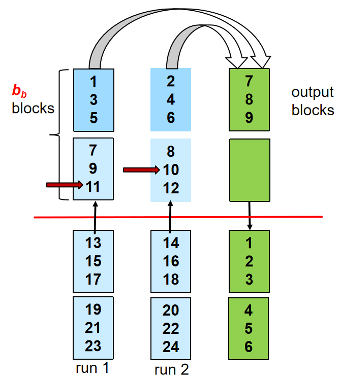
这样，一次可以把$\lfloor \frac{M}{b_b} \rfloor -1$个Runs合并为一个新的Runs

这样，一共需要的Pass数目为$P = \lceil \log_{\lfloor \frac{M}{b_b} \rfloor-1} (b_r /M) \rceil$

总的Block Transfers为:

\[ C = 2b_r \lceil \log_{\lfloor \frac{M}{b_b} \rfloor-1} {b_r / M} \rceil + b_r \]

总的Seek为:
- 在生成Runs时，也同样是Runs个数的两倍:$2 \lceil \frac{b_r}{M} \rceil$
- 不同的是，现在每个Pass中读和写的寻道个数都是$\lceil \frac{b_r}{b_b} \rceil$
- 所以总的寻道次数为:
  
  \[\begin{align} 2 \lceil \frac{b_r}{M} \rceil + 2\lceil \frac{b_r}{b_b} \rceil \lceil \log_{\lfloor \frac{M}{b_b} \rfloor-1} {b_r / M} \rceil - b_r \end{align}\]

Join Operation¶

我们使用的例子数据是:

Number of records of student:5,000,takes:10,000

Number of blocks of student:100,takes:400

我们希望完成$ r \bowtie_\theta s$

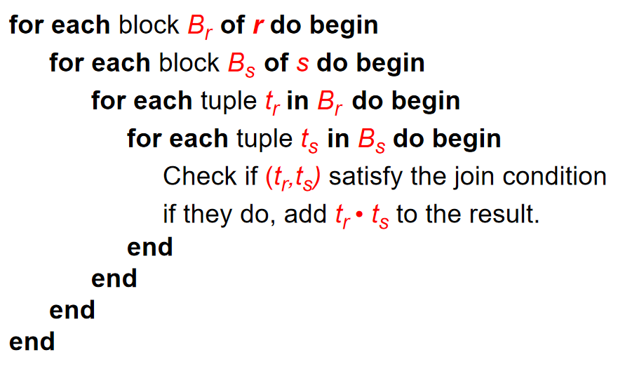
Nested-Loop Join¶

for each tuple tr in r do begin
    for each tuple ts in s do begin
        test pair (tr,ts) to see if they satisfy the join condition theta

        if they do, add tr • ts to the result.
    end
end

这是最朴素的做法
r 被称为outer relation，s 被称为inner relation.
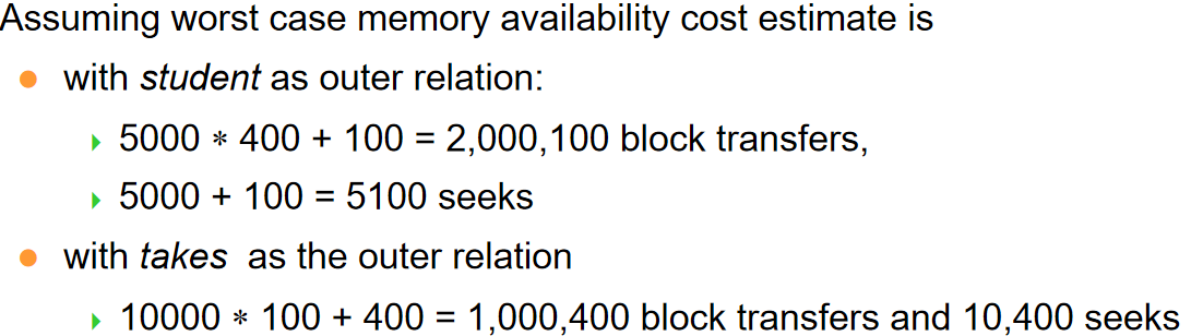
在最坏的情况，如果内存每次只能容纳两个关系各一个Block
- $n_r * b_s + b_r$次块传输
  - 因为r的每个元组都要和s的每个元组进行比较，所以r的一个元组要遍历s的所有块
- $n_r + b_r$次寻道(假设一个关系的块是连续存放的，每一个r的元组要Seek一次来找到s的块)
- $n_s$是关系s的元组数目
- $b_s$是关系s的块数目
- $b_r$是关系r的块数目
但是，如果有一个关系的元组足够少，少到能整个放进内存中
- 我们把这个关系当作内关系,始终放在内存中
- $b_r +b_s$次块传输
  - 因为我们只需要读一次内关系的所有块
- 两次寻道
  - 一次是读内关系的块，一次是读外关系的块

Block Nested-Loop Join¶

上一个算法的问题就在于，关系表中连续存放的元组在块中不一定是连续存放的，因此我们如果以块为单位读取，先读取块，再读这个块里面的元组，那就可以减少寻道次数与块传输次数。

相当于，我们先各读一个块，然后在内存中比较，相当于按块的顺序来比较

在这样的情况下，如果最坏:

$b_r * b_s + b_r$次块传输
- Each block in the inner relation s is read once for each block in the outer relation
$b_r + b_r$次寻道

最好的情况是一样的

Improvements to block nested loop algorithms:

假设内存有 M 块，有一块作为 output 的缓冲，剩下 M-1 块中 M-2 块均给外关系，内关系给一块。

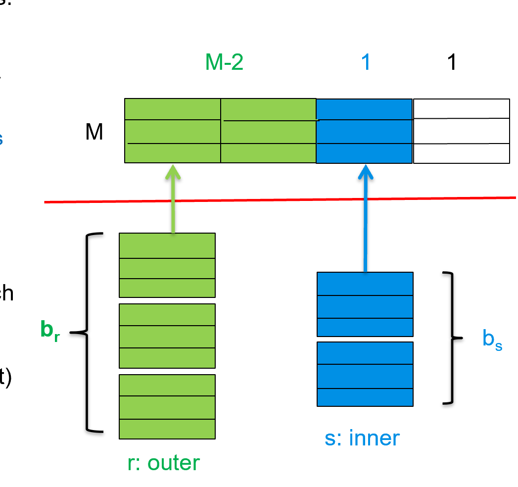
当然还是沿用块嵌套循环的思想

Block Transfers:$\lceil \frac{b_r}{M-2} \rceil * b_s + b_r$
Seek: $2 \lceil \frac{b_r}{M-2} \rceil$
- 假设对于外关系，一次读取连续的M-2块进来，这M-2块只需要一次寻道。
如果连接的属性是 key, 那么当我们匹配上之后就可以停止内循环。
利用 LRU 策略的特点，inner 正向扫描后再反过来，这样最近的块很可能还在内存中，提高缓冲命中率。

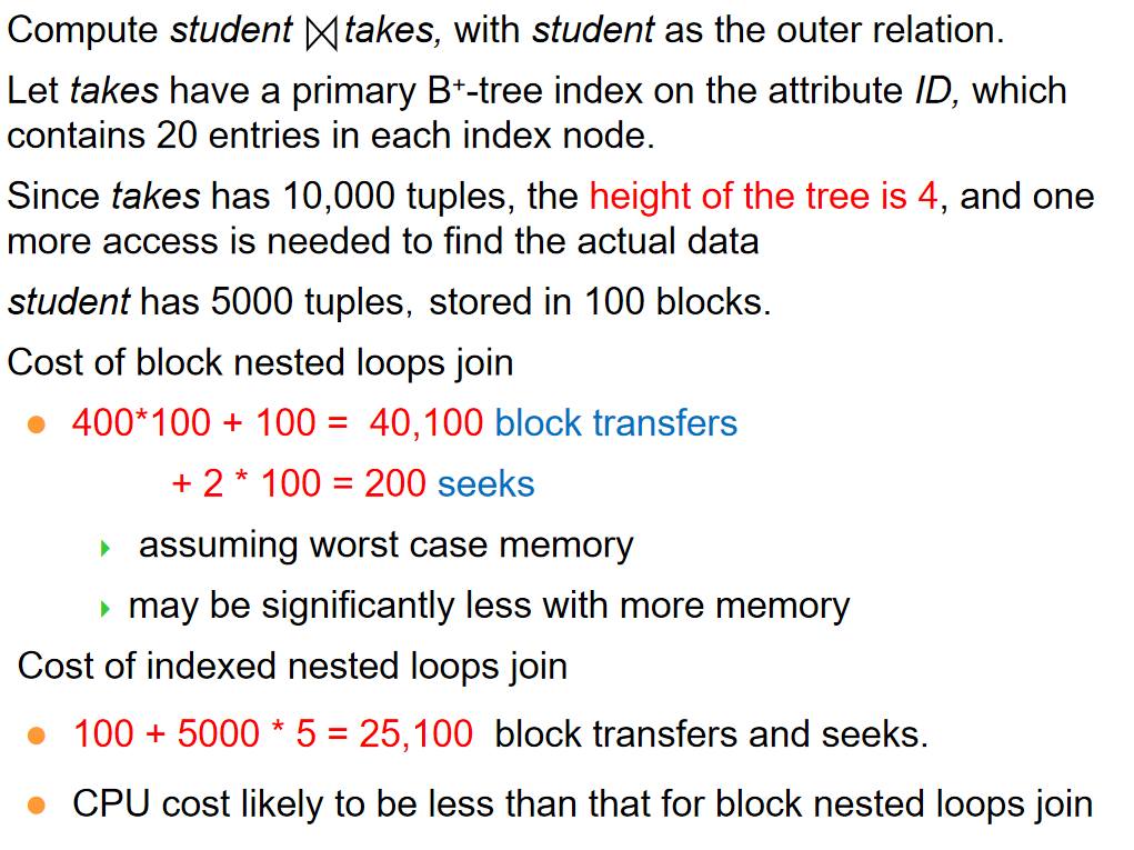
Indexed Nested-Loop Join¶

如果内循环的关系有索引，那么对于外循环的每一个元组，我们根据特定属性上的值在内循环的索引里查找。

Cost：$b_r (t_T + t_S) + n_r * c$

c指遍历索引并找到所有符合条件的元组的代价

🌰

Merge Join¶

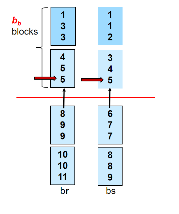
对于每一个关系，先按连接属性排好序
Merge the sorted relations to join them
- Join step is similar to the merge stage of the sort-merge algorithm.
- Main difference is handling of duplicate values in join attribute — every pair with same value on join attribute must be matched

由于每个块只需要传输一次，所以:

Block Transfers: $b_r + b_s$
Seek: $ \lceil \frac{b_r}{b_b} \rceil + \lceil \frac{b_s}{b_b} \rceil$

一个数学问题:如果内存有M块，如何分配给两个关系的块？

答案是: $$ x_r = \sqrt{b_r} \times \frac{M}{\sqrt{b_r} + \sqrt{b_s}}, \ x_s = \sqrt{b_s} \times \frac{M}{\sqrt{b_r} + \sqrt{b_s}} $$

Hash-Join¶

我们使用一个哈希函数，把元组分块，这样，由于哈希函数的特点，能够连接的属性的值一定在同一块中，反之不然。

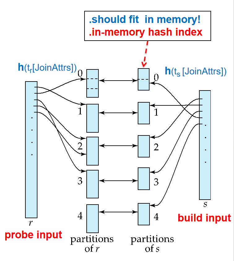
并且，分成的块数$n$与哈希函数要设计过，使得块的大小是足以放进内存的。

$n \geq \lceil \frac{b_s}{M} \rceil$

Hash-Join Algorithm¶

对关系s用哈希函数H，内存同样保留input buffer和output buffer，分片之后再写出去
关系r也用哈希函数H，分片之后再写出去
把s的第i个分块加载到内存中，并在连接属性上再用一个不同的哈希函数建立哈希索引
把r的第i个分块加载到内存中，每个元组在连接属性上作哈希，就能很快找到s中匹配的元组
把连接结果输出

因此，s被叫做build input，r被叫做probe input

修正因子

通常n会被选为$\lceil \frac{b_s}{M} \rceil *f$

其中f是修正因子，通常取1.2

需要注意的是，在分块的时候，我们要求对于每个块都要有一个输出缓冲块，比如哈希函数映射的值范围是0到n-1，那么我们就要有n个输出缓冲块,根据哈希函数的值来决定输出缓冲块的编号。

由此就引发了一个问题，因为这样的算法要求每次分块的个数必然不能大于内存的块数，如果原来关系很大，大到即使分成这么多块，大小还是太大了怎么办?

所以要用Recursive partitioning

Recursive partitioning¶

Instead of partitioning n ways, use M – 1 partitions for s
Further partition the M – 1 partitions using a different hash function
For example, consider a memory size of 12M bytes, divided into 4K bytes blocks; it would contain a total of 3K (3072) blocks. We can use a memory of this size to partition relations of size up to 3K ∗ 3K blocks, which is 36G (3K ∗ 3K ∗ 4K ) bytes.

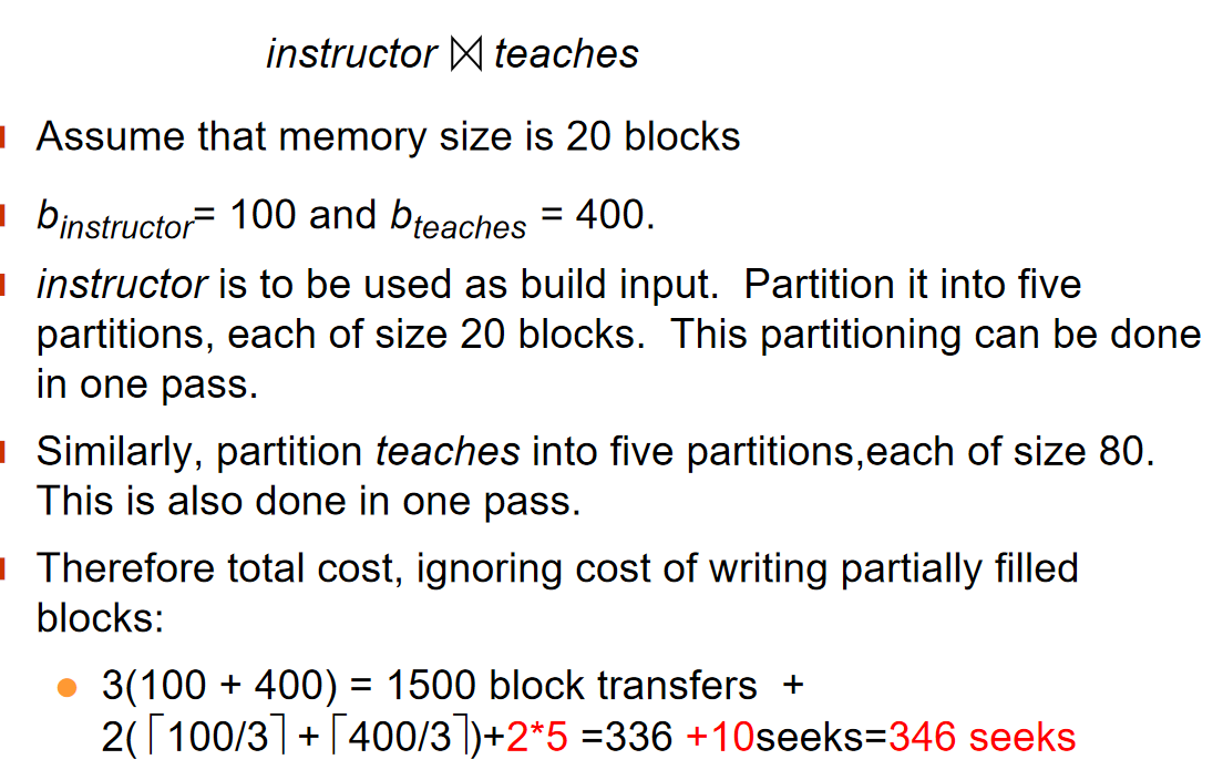
Cost of Hash Join¶

🌰

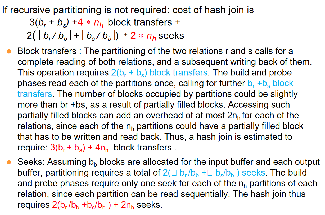
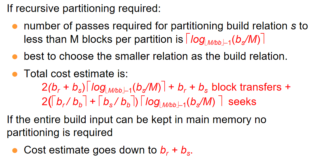
Other Operations¶

Duplicate elimination can be implemented via hashing or sorting.
- On sorting duplicates will come adjacent to each other, and all but one set of duplicates can be deleted.
- Optimization: duplicates can be deleted during run generation as well as at intermediate merge steps in external sort-merge.
- Hashing is similar – duplicates will come into the same bucket.
Aggregation can be implemented in a manner similar to duplicate elimination.
- Sorting or hashing can be used to bring tuples in the same group together, and then the aggregate functions can be applied on each group.
- Optimization: combine tuples in the same group during run generation and intermediate merges, by computing partial aggregate values
  - For count, min, max, sum: keep aggregate values on tuples found so far in the group.
    - When combining partial aggregate for count, add up the aggregates
  - For avg, keep sum and count, and divide sum by count at the end
集合操作
1. 对每个关系分块
2. 对于每个i，$r_i$建立哈希索引
  - 如果是取并集:
    - 如果$s_i$中的元组经过哈希函数映射后，值不存在，则加入哈希索引中
    - 输出哈希索引
  - 如果是取交集:
    - 如果$s_i$中的元组经过哈希函数映射后，值存在，就输出
  - 如果是取差集:
    - 如果$s_i$中的元组经过哈希函数映射后，值如果存在，就从哈希索引中删除
    - 输出哈希索引中的所有元组
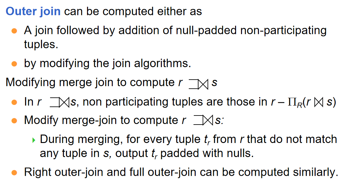
Outer Join