查询优化¶

约 3047 个字 15 行代码 29 张图片预计阅读时间 15 分钟

Introduction¶

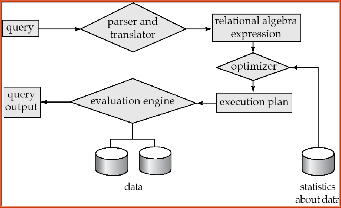
Alternative ways of evaluating a given query

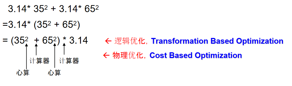
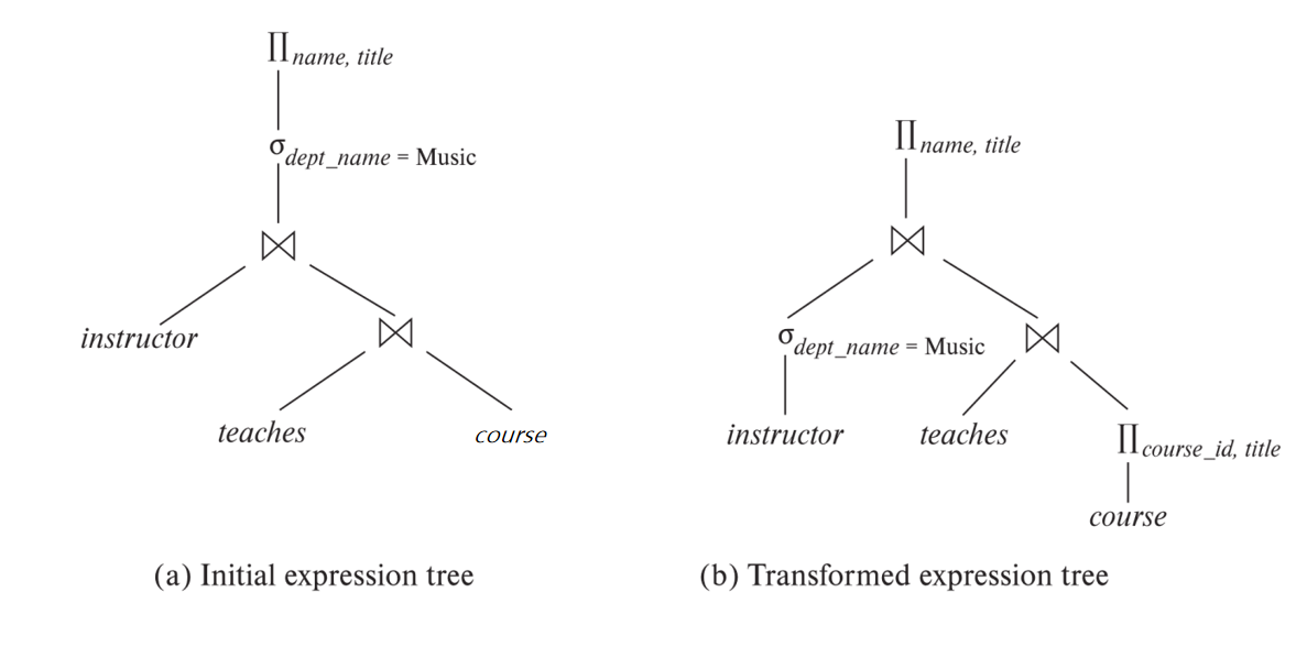
Equivalent expressions:逻辑优化，先做投影，选择
Different algorithms for each operation：物理层面的优化，为每个算子选择合适的算法

Example

Generating Equivalent Expressions¶

Two relational algebra expressions are said to be equivalent if the two expressions generate the same set of tuples on every legal database instance

Equivalence Rules¶

Selection¶

Conjunction decomposition: 选择条件可以分解成多个条件

\[\sigma_{p_1 \land p_2}(R) = \sigma_{p_1}(\sigma_{p_2}(R))\]
Selection commutativity: 选择条件可以交换

\[\sigma_{p_1}(\sigma_{p_2}(R)) = \sigma_{p_2}(\sigma_{p_1}(R))\]
Only the last projection is needed: 只需要最后的投影条件

\[\Pi_{L_1}(\Pi_{L2}(\dots(\Pi_{Ln}(R)))) = \Pi_{L1}(R)\]
Selections can be combined with Cartesian products and theta joins: 选择可以和笛卡尔积和连接结合

\[\sigma_{p_1}(R \times S) = R \bowtie_{p_1} S\]

\[\sigma_{p_1}(R \bowtie_{p_2} S) = R \bowtie_{p_1 \land p_2} S\]

Join¶

Join commutativity: 连接条件可以交换

\[R \bowtie_{p_1} S = S \bowtie_{p_1} R\]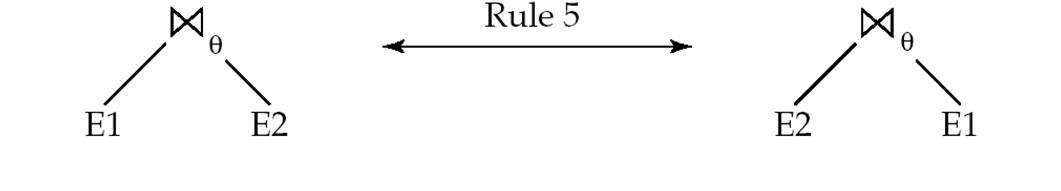
Join associativity: 连接条件可以结合
- $R \bowtie_{p_1} (S \bowtie_{p_2} T) = (R \bowtie_{p_1} S) \bowtie_{p_2} T$
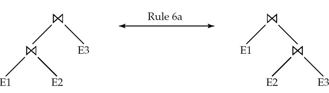
- 另一种神奇的结合是: $$ (R \bowtie_{p_1} S) \bowtie_{p_2 \land p_3} T = R \bowtie_{p_1 \land p_2} (S \bowtie_{p_3} T) $$
- 其中条件$p_3$包含只来自于S和T的属性
Select与Join分配
- $\sigma_{p_1}(R \bowtie_{p_2} S) = \sigma_{p_1}(R) \bowtie_{p_2} S$
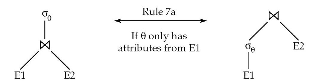
- $\sigma_{p_1 \land p_2}(R \bowtie_{p_3} S) = \sigma_{p_1}(R) \bowtie_{p_2} \sigma_{p_3}(S)$

Projection¶

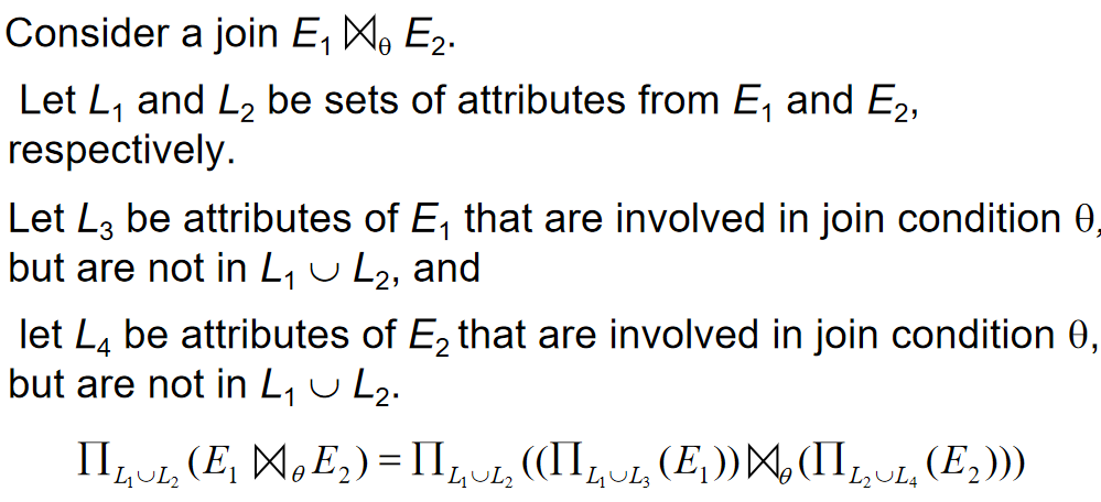
$\Pi_{L_1 \cup L_2}(R \bowtie_{p} S) = \Pi_{L_1}(R) \bowtie_{p} \Pi_{L_2}(S)$

集合操作¶

交换律
- $R \cup S = S \cup R$
- $R \cap S = S \cap R$
结合律
- $R \cup (S \cup T) = (R \cup S) \cup T$
- $R \cap (S \cap T) = (R \cap S) \cap T$
与Selection的分配律
- $\sigma_{\theta}(R \cup S) = \sigma_{\theta}(R) \cup \sigma_{\theta}(S)$
  - 对差集，交集同样成立
- $\sigma_{\theta}{R \cap S} = \sigma_{\theta}(R) \cap S$
  - 对差集成立，但是对于并集不成立
The projection operation distributes over union
- $\Pi_{L}(R \cup S) = \Pi_{L}(R) \cup \Pi_{L}(S)$

Other¶

Example

SelectProjectJoinMix

Enumeration of Equivalent Expressions¶

Repeat

apply all applicable equivalence rules on every subexpression of every equivalent expression found so far
add newly generated expressions to the set of equivalent expressions

Until no new equivalent expressions are generated above

Statistics for Cost Estimation¶

符号定义

$n_r$：relation r的元组数目
$b_r$：relation r的块数目
$l_r$: relation r一个元组的大小
$f_r$: r中一个block能存储的元组数目
$V(A,r)$: attribute A在relation r中不同值的个数,等价于$\Pi_{A}(r)$
If tuples of r are stored together physically in a file, then:
- $b_r = \lceil \frac{n_r}{f_r} \rceil$
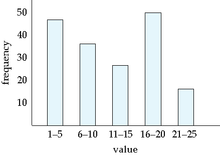
Histogram on attribute age of relation person

Selection Size Estimation¶

$\sigma_{A = v}(R) = \frac{1}{ V(A,r)} \cdot n_r$
- 这样的估算基于值是均匀分布的
- 如果A是主键,那么结果当然是1
$\sigma_{A \leq v}(R) $
- 令c为满足条件的元组数目
- c = 0 if $v < min(A,r)$
- $c= n_r \cdot \frac{v - min(A,r)}{max(A,r) - min(A,r)}$
- 如果没有最大最小值的统计,认为c是$\frac{V(A,r)}{2}$
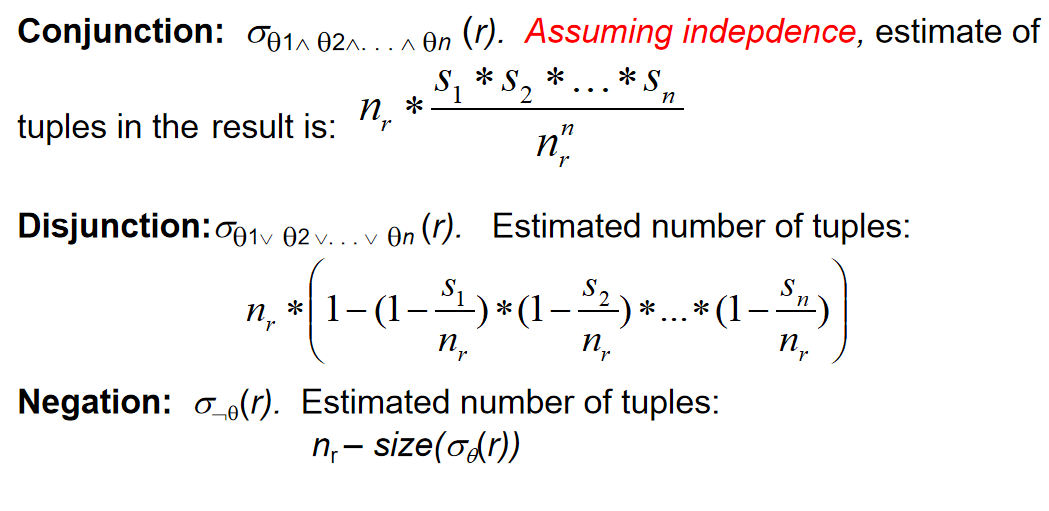
The selectivity（中选率）
- 对于某个条件$\theta_i$,它的中选率是r中的一个元组满足该条件的概率
- 令$s_i$是满足条件的元组数目,那么中选率是$s_i/n_r$
- 计算:

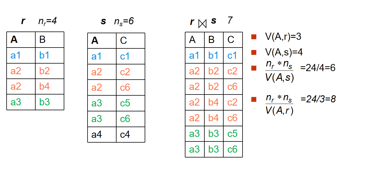
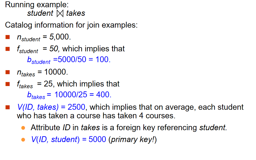
Estimation of the Size of Joins¶

对于笛卡尔乘积,结果的元组数目是$n_r \cdot n_s$

如果$R \cap S = \emptyset$,那么结果的元组数目是$n_r \cdot n_s$
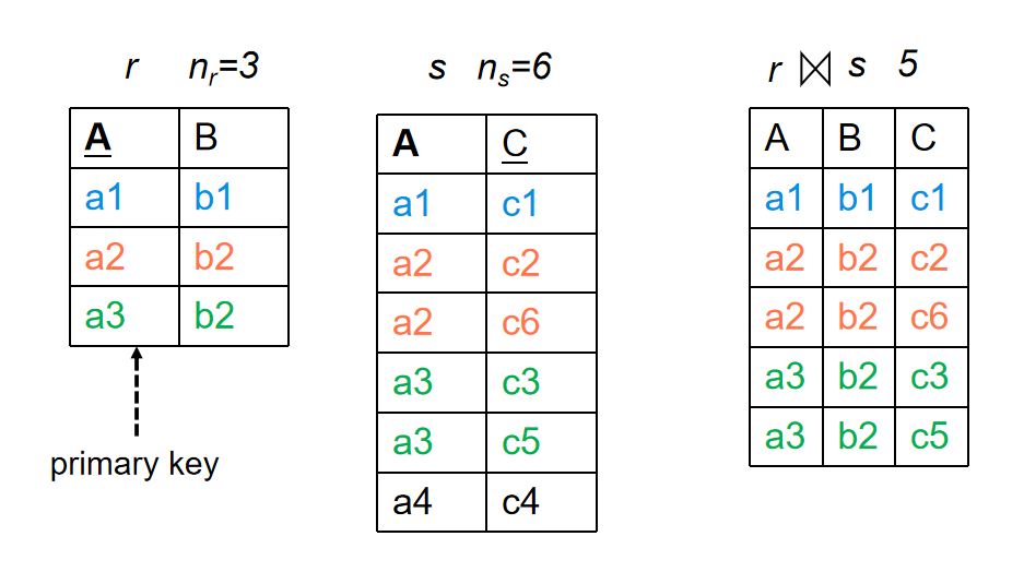
如果$R \cap S$的结果属性是R的主键,那么由于S中的一个元组最多和R中的一个元组连接,因此$R \bowtie S$的结果元组数目$\leq n_s$
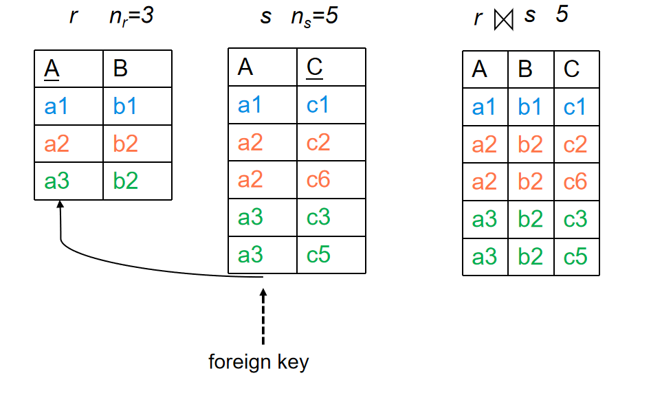
如果$R \cap S$的结果属性是S引用R的外键,那么结果的元组数目就是$n_s$
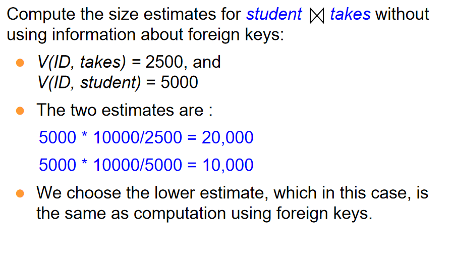
如果$R \cap S$的结果属性都不是上面的情况
- If we assume that every tuple t in R produces tuples in $R \bowtie S$,那么元组数目是
  
  \[\frac{n_r \cdot n_s}{V(A,s)}\]
- 相当于计算每个R中的元组可以与S中的几个元组连接
- 反之,公式是
  
  \[\frac{n_r \cdot n_s}{V(A,r)}\]

Example

Size Estimation for Other Operations¶

Projection: 估计$\Pi_{A}(R)$的结果元组数目是$V(A,r)$
Aggregation: 估计$\gamma_{A}(R)$的结果元组数目是$V(A,r)$
Set operations:
- For unions/intersections of selections on the same relation: rewrite and use size estimate for selections
- 比如:
  
  \[\sigma_{\theta_1}(R) \cup \sigma_{\theta_2}(R) = \sigma_{\theta_1 \lor \theta_2}(R)\]
- 对于直接的集合操作:
  - $\cup$ : $n_r + n_s$
  - $\cap$: $min(n_r, n_s)$
  - $r-s$: $n_r$
  - All the three estimates may be quite inaccurate, but provide upper bounds on the sizes.
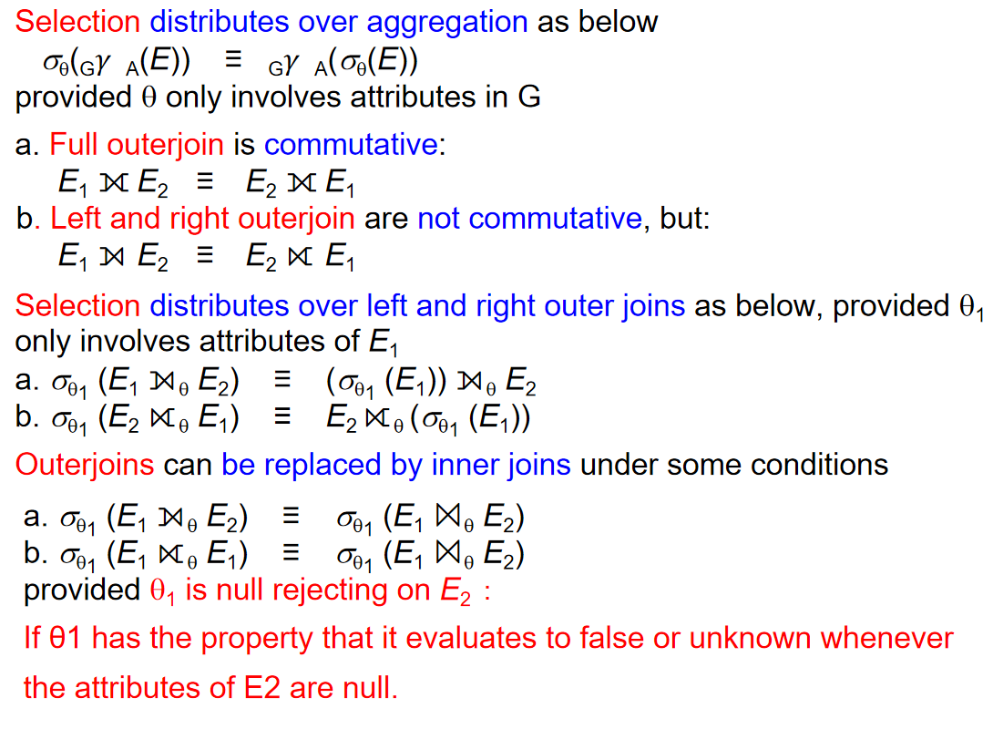
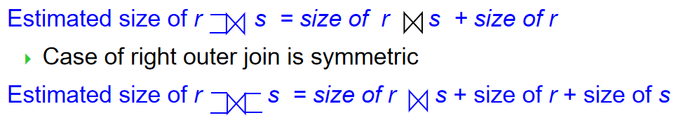
Outer Join

Estimation of Number of Distinct Values¶

上面许多估计都要用到$V(A,r)$,即relation r中属性A的不同值的个数

Selection,estimate $V(A,\sigma_{\theta}(R))$
- If $\theta$ forces A to take a specified value: $V(A,\sigma_{\theta}(R))$ = 1.
  - e.g., A = 3
- If $\theta$ forces A to take on one of a specified set of values:
  - $V(A,\sigma_{\theta}(R))$= number of specified values.
  - (e.g., (A = 1 V A = 3 V A = 4 )),
- If the selection condition  is of the form A op v
  - estimated $V(A,\sigma_{\theta}(R))$ = $V(A,r) \dot s$
  - s是上面说的中选率
- In all the other cases, use approximate estimate:
  - $V(A,\sigma_{\theta}(R)) = min(V(A,r), n_{\sigma_\theta (r)} )$
Join,estimate $V(A,r\bowtie s)$
- 如果A的所有属性来自R,那么$V(A,r \bowtie s) = min(V(A,r), n_{r \bowtie s})$
- 如果A包含来自r的属性A1和来自s的属性A2，那么$V(A,r \bowtie s) = min(V(A1,r)*V(A2-A1,s), V(A1-A2,r)*V(A2,s),n_{r \bowtie s})$
Projection and aggregation

Choice of Evaluation Plans¶

Must consider the interaction of evaluation techniques when choosing evaluation plans

choosing the cheapest algorithm for each operation independently may not yield best overall algorithm. E.g.
- merge-join may be costlier than hash-join, but may provide a sorted output which reduces the cost for an outer level aggregation.就是说，归并的代价可能暂时很大，但是这样做了可以减少后续操作的开销
- nested-loop join may provide opportunity for pipelining

Cost-Based Join-Order Selection¶

对于$r_1 \bowtie r_2 \cdots \bowtie r_n$，我们需要选择一个恰当的顺序来使得代价最小

一共有$\frac{(2(n-1))!}{(n-1)!}$种可能的顺序

但正如下面这个例子:

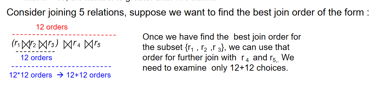
我们实际上可以用动态规划的思想来找到最佳的排列顺序

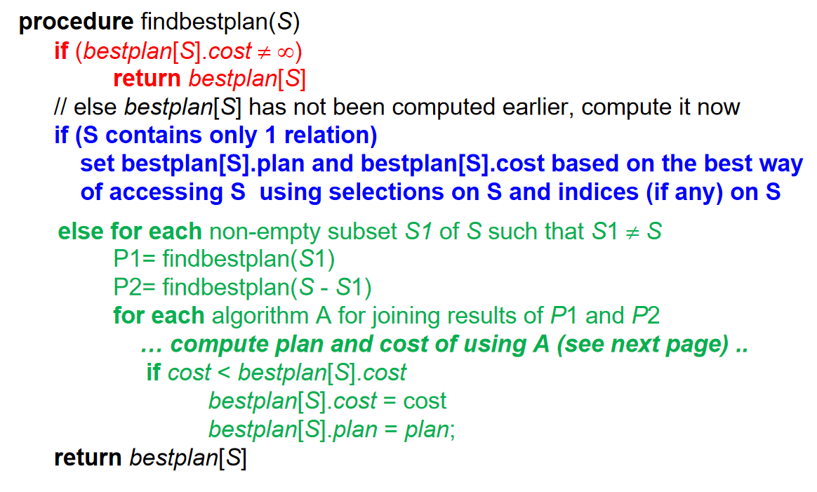
递归到最深就是单个表，对于单个表，我们用Select和Index找到最佳的代价
正常就是遍历所有可能把原来的表拆分为两个子表的情况($2^n-2$，两个有空集的情况不算)，然后再递归计算子表的代价。

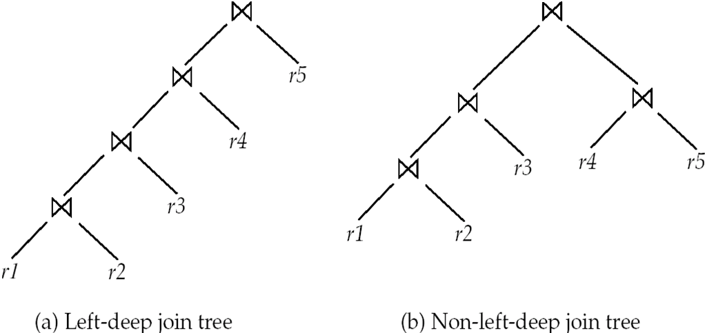
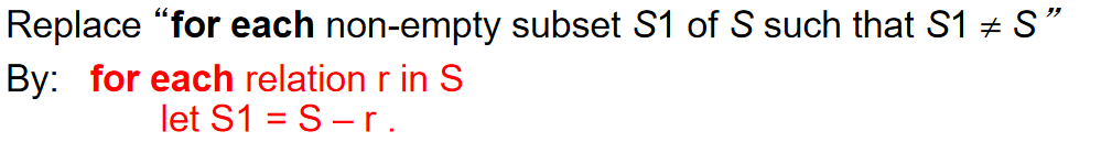
Left Deep Join Trees¶

In left-deep join trees, the right-hand-side input for each join is a relation, not the result of an intermediate join.

Cost of Optimization¶

Dynamic Programming
- 需要O(n^3)的时间来计算最优的连接顺序
- 需要O(n^2)的空间来存储中间结果
left-deep join tree
- 需要$O(n2^n)$的时间来计算最优的连接顺序
- 需要$O(2^n)$的空间来存储中间结果

Heuristic Optimization(启发式优化)¶

Heuristic optimization transforms the query-tree by using a set of rules that typically (but not in all cases) improve execution performance:

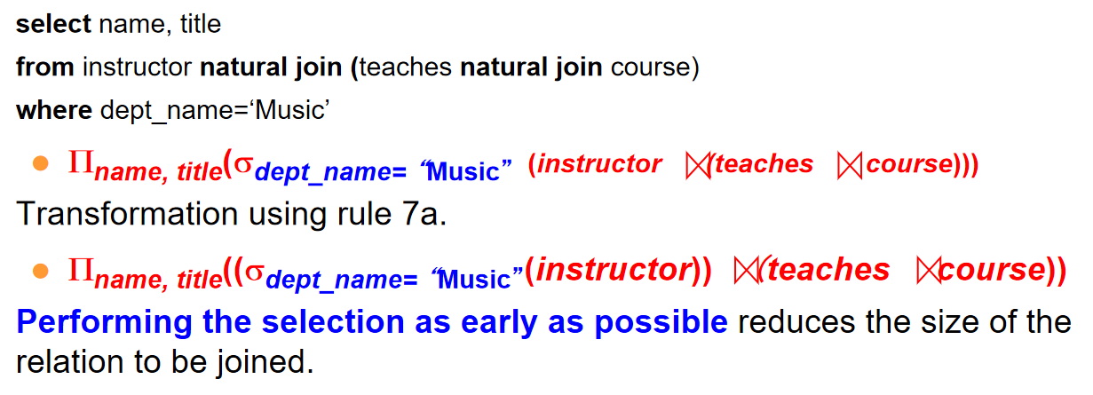
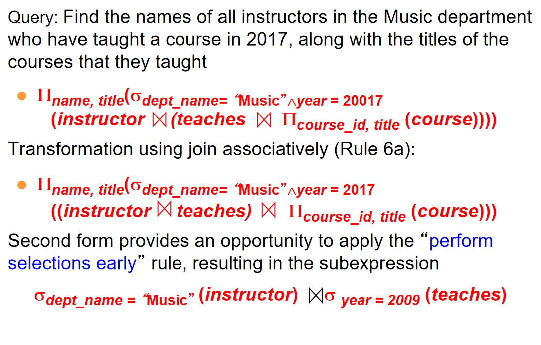
Perform selection early (reduces the number of tuples)
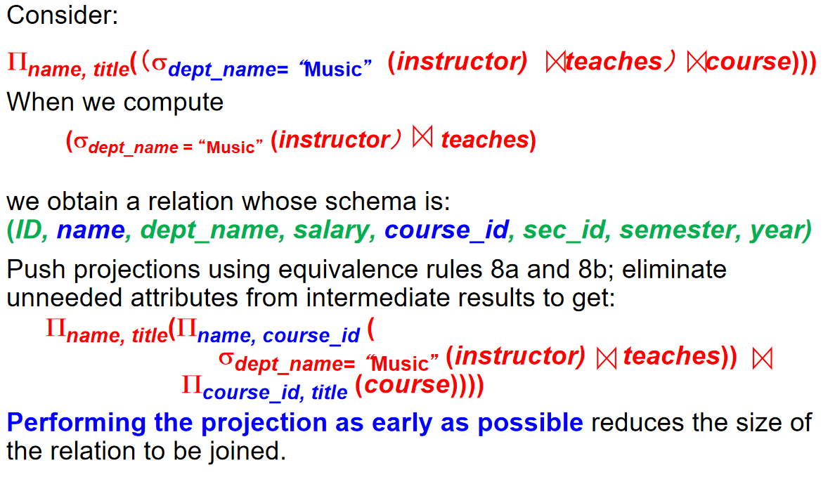
Perform projection early (reduces the number of attributes)
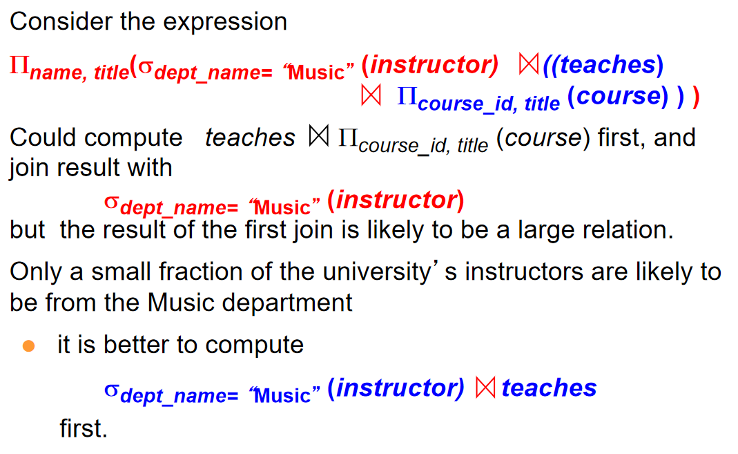
Perform most restrictive selection and join operations (i.e. with smallest result size) before other similar operations.
Perform left-deep join order
Some systems use only heuristics, others combine heuristics with partial cost-based optimization.

Additional Optimization Techniques¶

Optimizing Nested Subqueries¶

对于如下的嵌套查询:

select name 
from instructor
where exists (select *
        from teaches
        where instructor.ID = teaches.ID and teaches.year = 2022)

这相当于是一个两重循环,低效.

Parameters are variables from outer level query that are used in the nested subquery; such variables are called correlation variables（相关变量）

比如上面的例子中,instructor.ID就是一个相关变量

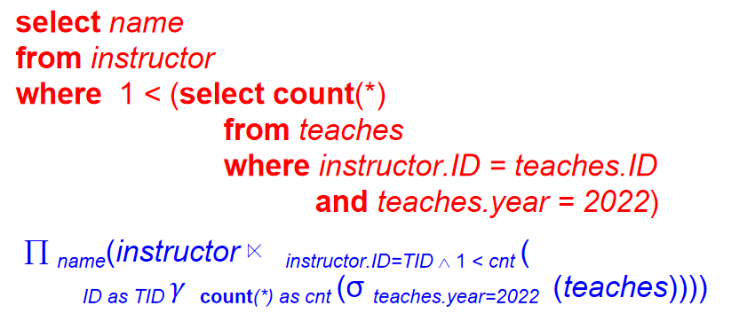
我们想要把这个查询变得高效.常见的做法是把内层的查询变成一个连接操作,然后再做投影.也就是把上面的查询变成:

select name
from instructor, teaches
where instructor.ID = teaches.ID and teaches.year = 2022

但是,这样的做法还有问题.teaches中可能有许多重复的ID,这样就会导致instructor中的元组被重复计算,从而导致不必要的开销.

为解决这个问题,我们可以使用半连接(semijoin)来避免重复计算.

Semijoin

半连接的符号是$\ltimes$,其定义如下:

"If a tuple $r_i$ appears n times in r, it appears n times in the result of $r \ltimes_\theta s$ , if there is at least one tuple $s_i$ in s matching with $r_i$"

通俗来讲,半连接就是连接操作,但是只保留左表的元组,而不保留右表的元组.也就是说,半连接的结果是左表中所有满足条件的元组,而不是连接后的结果.

这样,我们就可以把上面的查询变成:

\[\Pi_{name}(instructor \ltimes_{instructor.ID = teaches.ID \land teaches.year=2022} teaches)\]

这样重复的名字就不会被多次计算,同时也可以避免同名出现问题.

因此,我们可以说,形如:

SELECT A
FROM r_1, r_2, ..., r_n
WHERE P_1 AND EXISTS (
    SELECT *
    FROM s_1, s_2, ..., s_m
    WHERE P_2^1 AND P_2^2
)

可以改写为:

\[ \Pi_A\left( \sigma_{P_1}(r_1 \times r_2 \times \cdots \times r_n) \ltimes_{P_2^2} \sigma_{P_2^1}(s_1 \times s_2 \times \cdots \times s_m) \right) \]

其中：

$ P_2^1 $ 包含不涉及外层查询变量的谓词（简单条件）。
$ P_2^2 $ 包含涉及外层查询变量的谓词（相关子查询条件）。
将一个嵌套子查询替换为一个带有连接或半连接的查询（可能涉及临时表），这个过程称为 Decorrelation（去除相关性）。

在以下情况下，去相关化过程会更加复杂：

嵌套子查询中使用了聚合操作，或
嵌套子查询是一个标量子查询（返回单个值）。

这时通常需要使用相关性评估（Correlated Evaluation）。

Example

Materialized Views¶

之前讲过,物化视图就是把原来的视图变成一个真正的表,这样在查询的时候就可以直接查询这个表,而不需要每次都去计算视图.

但是,这样做也是有代价的,我们需要在原来的表发生变化的时候,去更新这个物化视图,这样就会导致额外的开销.

这样的工作被称为materialized view maintenance

一个好的办法是incremental view maintenance(增量视图维护)~~感觉和latex与typst的区别差不多~~

视图维护可以通过以下方法操作:

使用trigger来维护视图,当原来的表发生变化的时候,就会触发一个trigger,然后去更新物化视图.
手动写一个更新程序
定时更新,比如晚上

The changes (inserts and deletes) to a relation or expressions are referred to as its differential（差分）

差分就是差异

Join Operation
- 如果物化视图$v = r \bowtie s$,并且更新r
- 我们把原来和更新后的表称为$r_{new}$和$r_{old}$,那么:
  - 对于插入,$r_{new} \bowtie s = (r_{old} \cup i_r) \bowtie s$
  - 也即$r_{old} \bowtie s \cup i_r \bowtie s$,$r_{old} \bowtie s$是原来的视图,而$i_r \bowtie s$是新插入的元组和s连接的结果,也就是增量
  - 故$v_{new} = v_{old} \cup i_r \bowtie s$
  - 删除同理,是$v_{old} - d_r \bowtie s$
Selection : $v = \sigma_{p}(r)$
- 插入: $v_{new} = v_{old} \cup i_r$
- 删除: $v_{new} = v_{old} - d_r$
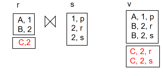
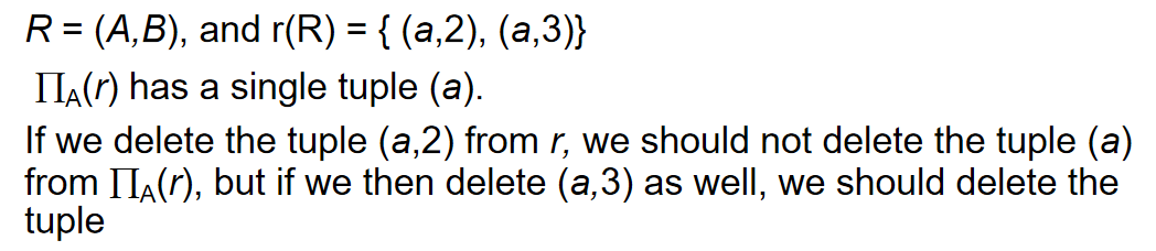
Projection,more difficult
- 对于每一个$\Pi_{A}(r)$,我们维护其每个元组被取回次数
- r插入了一个元组,如果它的映射已经在视图中,那么我们就增加这个元组的计数,如果它的映射不在视图中,那么我们就把计数置1,并且把它加入到视图中
- 同理,删除的时候我们就减少这个元组的计数,如果计数为0,那么我们就把它从视图中删除
Count: $v =_A \gamma_{count(B)}(r)$
- 当向原表中插入一组元组 ir 时：
  - 对于 ir 中的每个元组r：
    - 首先检查它在对应的组是否已经存在于视图 v 中
    - 如果该组已存在，就将该组的计数增加 1
    - 如果该组不存在，就添加一个新的元组到视图中，并设置计数为 1
- 当从原表中删除一组元组 dr 时：
  - 对于 dr 中的每个元组：
    - 在视图 v 中查找它的组
    - 将该组的计数减少 1
    - 如果计数变为 0，表示原表中不再有任何元组投影到这个值，因此从视图 v 中删除该组
sum: $v =_A \gamma_{sum(B)}(r)$
- 和count类似,但是我们需要维护每个组的和,而不是计数
- 插入的时候,我们就把这个元组的值加到视图中,删除的时候就减去这个元组的值
- 同时,我们也需要维护count,以便当检测到一个组中没有元组时,把这个组删去,而不是简单地判断它的sum是不是0
- 维护了sum和count,我们也可以算出avg了
min,max,删除时比较复杂
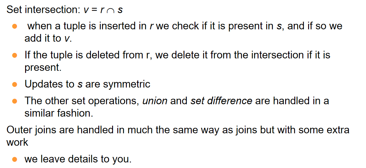
集合操作

Materialized View Selection¶

What is the best set of views to materialize?

查询优化¶

Introduction¶

Generating Equivalent Expressions¶

Equivalence Rules¶

Selection¶

Join¶

Projection¶

集合操作¶

Other¶

Enumeration of Equivalent Expressions¶

Statistics for Cost Estimation¶

Selection Size Estimation¶

Estimation of the Size of Joins¶

Size Estimation for Other Operations¶

Estimation of Number of Distinct Values¶

Choice of Evaluation Plans¶

Cost-Based Join-Order Selection¶

Left Deep Join Trees¶

Cost of Optimization¶

Heuristic Optimization(启发式优化)¶

Additional Optimization Techniques¶

Optimizing Nested Subqueries¶

Materialized Views¶

Materialized View Selection¶

评论